How to Highlight Every Other Row in Excel (Complete Guide for IT Professionals)

1. Introduction

When working with large datasets in Excel, readability becomes a serious challenge. Rows start blending together, making it harder to track values across columns—especially in financial reports, logs, or datasets with hundreds of entries.

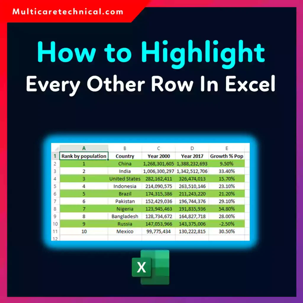
That’s where highlighting every other row (also called banded rows or zebra striping) comes in. This simple formatting technique dramatically improves readability, reduces errors, and makes your spreadsheets look more professional.

Whether you’re a beginner or an IT professional managing complex data, this guide will walk you through multiple methods to highlight alternating rows in Excel, along with pro tips and troubleshooting techniques.

2. Quick Answer (Featured Snippet)

To highlight every other row in Excel:

1. Select your data range
2. Go to Home → Conditional Formatting → New Rule
3. Choose Use a formula to determine which cells to format
4. Enter this formula: =MOD(ROW(),2)=0
5. Click Format, choose a fill color, and press OK

This will highlight every even row. Use =MOD(ROW(),2)=1 for odd rows.

3. Table of Contents

• What Does Highlighting Alternate Rows Mean?
• Why It’s Important for Data Management
• Method 1: Conditional Formatting (Best Method)
• Method 2: Format as Table
• Method 3: Manual Formatting (Not Recommended)
• Step-by-Step Detailed Guide
• Common Errors and Fixes
• Best Practices and Pro Tips
• FAQs
• Conclusion

4. Explanation Section

What Does Highlighting Every Other Row Mean?

Highlighting every other row means applying a background color to alternating rows (e.g., rows 2, 4, 6, etc.). This creates a striped effect that makes it easier to visually scan data.

Why Is It Important?

• Improves readability of large datasets
• Reduces data entry and analysis errors
• Makes reports look professional
• Helps in presentations and dashboards

For IT professionals working with logs, exports, or reports, this technique is essential.

5. Step-by-Step Guide

Method 1: Conditional Formatting (Recommended)

This is the most flexible and widely used method.

Step 1: Select Your Data

Highlight the range where you want to apply formatting (e.g., A1:D100).

Step 2: Open Conditional Formatting

Go to:
Home → Conditional Formatting → New Rule

Step 3: Choose Formula Option

Select:
“Use a formula to determine which cells to format”

Step 4: Enter the Formula

For even rows:

=MOD(ROW(),2)=0

For odd rows:

=MOD(ROW(),2)=1

Step 5: Choose Formatting

Click Format → Fill tab → Select a color

Step 6: Apply

Click OK → OK

✅ Done! Your rows will now be automatically highlighted.

Method 2: Format as Table (Fastest Way)

If you’re looking for a quick solution:

Steps:

1. Select your data
2. Press Ctrl + T
3. Choose a table style
4. Ensure Banded Rows is checked

Excel automatically applies alternating colors.

💡 Bonus: Tables also give you sorting and filtering options.

Method 3: Manual Formatting (Basic)

This method is not recommended for large datasets.

Steps:

1. Select a row
2. Apply a fill color
3. Skip one row and repeat

❌ Problem: Not dynamic—doesn’t update automatically when data changes.

6. Common Errors and Fixes

❌ Formula Not Working

Problem: No rows are highlighted
Fix:

• Ensure you typed the formula correctly
• Check if you selected the correct range

❌ Wrong Rows Highlighted

Problem: Odd rows instead of even (or vice versa)
Fix:

• Switch between:
  • =MOD(ROW(),2)=0
  • =MOD(ROW(),2)=1

❌ Formatting Breaks After Sorting

Problem: Colors don’t follow rows after sorting
Fix:

• Always apply formatting to the entire dataset
• Use Excel Tables for dynamic behavior

❌ Header Row Gets Highlighted

Problem: Header is also colored
Fix:

• Start selection from row 2 instead of row 1
• Or adjust formula: =MOD(ROW()-1,2)=0

7. Best Practices / Pro Tips

✔ Use Excel Tables for Dynamic Data

Tables automatically maintain alternating colors when you add or remove rows.

✔ Choose Light Colors

Use subtle shades like light gray or light blue to maintain readability.

✔ Combine with Filters

Alternating rows work great with filters and sorting—especially for dashboards.

✔ Apply to Entire Columns

Instead of selecting a fixed range, apply formatting to full columns for scalability.

✔ Use Named Ranges (Advanced Users)

For complex sheets, combine conditional formatting with named ranges for better control.

✔ Keep Data Clean

Before formatting, ensure your data is structured properly. For example, if you’re dealing with names, you can learn how to organize them here:
👉 https://multicaretechnical.com/how-to-separate-names-in-excel-step-by-step-guide-for-beginners-it-professionals

✔ Duplicate Sheets Before Editing

Always create a backup before applying formatting changes:
👉 https://multicaretechnical.com/how-to-make-a-copy-of-an-excel-sheet-step-by-step-guide-for-beginners-it-pros

✔ Stay Secure with Data Sources

If you’re importing data from external links, understand security best practices:
👉 https://multicaretechnical.com/how-should-you-approach-a-compressed-url-complete-security-guide

8. FAQs

1. How do I highlight every third row in Excel?

Use this formula:

=MOD(ROW(),3)=0

2. Can I apply different colors to alternating rows?

Yes. You can create multiple conditional formatting rules with different formulas.

3. Does this work in Excel Online?

Yes, conditional formatting works in Excel Online, though some advanced features may vary.

4. How do I remove alternating row formatting?

Go to:
Home → Conditional Formatting → Clear Rules

5. Can I apply this to columns instead of rows?

Yes. Use:

=MOD(COLUMN(),2)=0