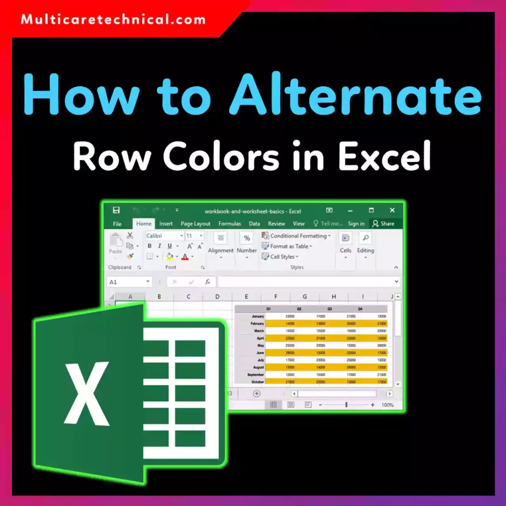
Long spreadsheets can get hard to read fast. Alternating row colors—also called banded rows—make Excel data easier to scan, reduce mistakes, and give your sheets a clean, professional look.
In this guide, you’ll learn how to alternate row colors in Excel automatically, with or without tables, on Windows, Mac, and Pivot Tables—even if your sheet has no header.

Why Alternate Row Colors in Excel?
Alternating row colors help you:
- Read large datasets faster
- Avoid row-tracking errors
- Make reports look professional
- Improve usability for teams
If Excel behaves strangely while navigating rows, this quick fix may help:
👉 How to disable Scroll Lock in Excel (Windows & Mac)
How to Alternate Row Colors in Excel Table (Easiest Method)
This is the fastest and most beginner-friendly option.
Steps:
- Select your data
- Go to Home → Format as Table
- Choose any table style
- Click OK
✔ Excel automatically applies alternating row colors
✔ Colors adjust automatically when rows are added
This method works best when you don’t mind converting data into a table.
How to Alternate Row Colors in Excel Automatically (Conditional Formatting)
Want automation without turning data into a table? Use conditional formatting.
Steps:
- Select the data range
- Go to Home → Conditional Formatting → New Rule
- Choose Use a formula
- Enter:
=MOD(ROW(),2)=0 - Pick a fill color → Click OK
✔ Works dynamically
✔ Updates as rows are added or removed
This is the best method for how to alternate row colors in Excel without formatting as table.
How to Alternate Row Colors in Excel Without Table
If you want clean formatting without table features:
- Use Conditional Formatting (recommended)
- Or manually apply alternating fills (static)
⚠ Manual formatting won’t update automatically.
How to Alternate Row Colors in Excel Without Conditional Formatting
If you prefer a manual approach:
Steps:
- Select every other row manually
- Apply a fill color
- Repeat for remaining rows
✔ Works offline
❌ Not dynamic
❌ Not ideal for large datasets
This method suits small, fixed spreadsheets.
How to Alternate Row Colors in Excel Without Header
No headers? No problem.
- Select only the data rows
- Apply Conditional Formatting or Format as Table
- Disable Header Row from Table Design (if using a table)
✔ Colors apply cleanly without affecting layout.
How to Alternate Row Colors in Excel Mac
Excel for Mac supports all main methods.
Best Options on Mac:
- Format as Table
- Conditional Formatting using ROW() formula
Steps are nearly identical to Windows versions.
How to Alternate Row Colors in Excel Pivot Table
Pivot tables need a slightly different approach.
Steps:
- Click inside the Pivot Table
- Go to Design
- Check Banded Rows
- Choose a Pivot Table style
✔ Automatically updates when Pivot refreshes
✔ Best for reports and dashboards
If your Pivot is locked, you may need to unprotect it first:
👉 How to unprotect a sheet in Excel with or without password
Pro Tips for Better Excel Formatting
- Use light colors to avoid eye strain
- Keep contrast consistent
- Avoid dark fills for printed sheets
- Combine with interactive elements like checkboxes
For task trackers, this guide pairs perfectly:
👉 How to add a checkbox in Excel (Windows, Mac, 2016–2019)
Frequently Asked Questions (Quick Answers)
How do I alternate row colors in Excel automatically?
Use Format as Table or Conditional Formatting with the ROW() formula.
Can I alternate row colors without a table?
Yes, Conditional Formatting works perfectly without tables.
Does this work on Excel Mac?
Yes, all major methods work on Excel for Mac.
Can Pivot Tables have alternating row colors?
Yes, enable Banded Rows from the Pivot Table Design tab.
Conclusion
Now you know how to alternate row colors in Excel using every method—tables, conditional formatting, Mac, Pivot Tables, and manual styles. Whether you want full automation or simple visual clarity, alternating colors instantly improves readability and professionalism.
Choose the method that fits your workflow—and make your spreadsheets easier to use.