
Microsoft Excel makes it easy to highlight important information, identify problems, and analyze data using colors. But what if you want Excel to change the color of one cell based on the value in another cell? For example, you might want a sales figure to turn green when a target is achieved, a task name to turn red when its deadline has passed, or an entire row to be highlighted when a status column contains “Pending.”
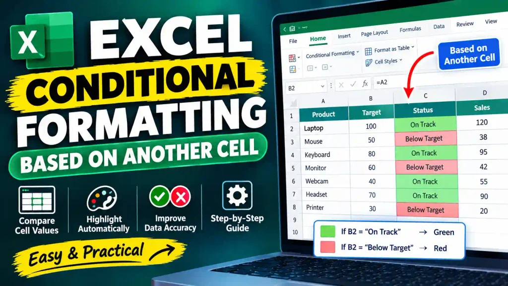
You can accomplish all these tasks with Excel conditional formatting based on another cell. By creating a rule with a formula, you can automatically format cells or entire rows according to values elsewhere in your worksheet.
In this guide, you’ll learn how to create conditional formatting rules in Excel for Windows and Mac, use relative and absolute cell references, highlight entire rows, troubleshoot common errors, and apply practical examples to real-world spreadsheets.
Quick Answer: How to Apply Conditional Formatting Based on Another Cell
To apply conditional formatting based on another cell in Excel:
- Select the cells you want to format.
- Go to Home > Conditional Formatting > New Rule.
- Select Use a formula to determine which cells to format.
- Enter a formula that references the cell containing the condition.
- Click Format, choose your preferred formatting, and click OK.
For example, to highlight cell A2 when B2 contains the word Completed, use:
=$B2="Completed"
If you apply this rule to A2, Excel will check the corresponding cell in column B for each row and highlight the matching cells.
Important: The formula must return TRUE for the formatting to be applied. Use the correct cell references for your selected range.
Table of Contents
- What is conditional formatting based on another cell?
- Example 1: Highlight a cell based on another cell’s text
- Example 2: Highlight an entire row based on a cell value
- Example 3: Compare two cells and highlight differences
- Example 4: Highlight dates based on another cell
- Example 5: Highlight values based on a number in another cell
- Relative and absolute cell references explained
- Common errors and fixes
- Best practices and pro tips
- Frequently asked questions
- Conclusion
What Is Conditional Formatting Based on Another Cell?
Conditional formatting is an Excel feature that automatically changes the appearance of cells when specified conditions are met.
You can use it to change a cell’s background color, font color, font style, or border based on a value in another cell.
For example, imagine you have a sales report with three columns:
| Product | Sales Target | Actual Sales |
|---|---|---|
| Laptop | 100 | 120 |
| Mouse | 50 | 38 |
| Keyboard | 80 | 95 |
| Monitor | 60 | 42 |
You want to highlight actual sales in green when they meet or exceed the target and red when they fall below it.
Excel can compare the values in columns B and C automatically. You do not need to manually color individual cells or update the formatting whenever the numbers change.
The same approach works for project tracking, attendance sheets, inventory management, expense reports, employee performance, and many other business tasks.
Example 1: Highlight a Cell Based on Another Cell’s Text
Suppose column A contains employee names and column B contains their work status. You want the employee’s name to turn green whenever the status is “Completed.”
| Employee | Status |
|---|---|
| John | Completed |
| Sarah | Pending |
| Michael | Completed |
| Emily | In Progress |
Follow these steps.
Step 1: Select the cells to format
Select the employee names in A2, or select the smaller range containing your actual data.
Step 2: Create a conditional formatting rule
Go to Home > Conditional Formatting > New Rule.
In the New Formatting Rule window, choose Use a formula to determine which cells to format.
Step 3: Enter the formula
Enter this formula:
=$B2="Completed"
The formula checks column B for the word “Completed.” The dollar sign before B keeps the reference in column B while the row number adjusts for each selected cell.
Step 4: Choose the formatting
Click Format, open the Fill tab, and select a green background. You can also choose a font color or bold text.
Click OK, and then click OK again to save the rule.
Now the employee names will be highlighted when their corresponding status is “Completed.”
You can replace "Completed" with "Pending", "Approved", "Rejected", or another status that matches your worksheet.
Example 2: Highlight an Entire Row Based on a Cell Value
Highlighting an entire row is useful when you manage large lists of orders, projects, employees, or inventory items.
Suppose your worksheet has the following columns:
| Task | Assigned To | Due Date | Status |
|---|---|---|---|
| Website update | John | 10/15/2026 | Completed |
| Server backup | Sarah | 10/18/2026 | Pending |
| Security review | Michael | 10/20/2026 | In Progress |
You want the entire row to turn green whenever the status in column D is “Completed.”
Step-by-step instructions
- Select the data range
A2:D100. - Go to Home > Conditional Formatting > New Rule.
- Select Use a formula to determine which cells to format.
- Enter this formula:
=$D2="Completed" - Click Format and select a green fill color.
- Click OK to apply the rule.
Excel will check column D for each row and highlight all cells in that row when the status is “Completed.”
Why does the formula use $D2?
The dollar sign locks the column reference to D, while the row number remains relative.
This means Excel checks D2 for the first row, D3 for the second row, D4 for the third row, and so on.
If you want to highlight rows with a status of “Pending,” use:
=$D2="Pending"
Choose a red or yellow fill to make those tasks easier to identify.
Example 3: Compare Two Cells and Highlight Differences
Conditional formatting can compare values in two cells and highlight the result when they differ.
Suppose column A contains expected quantities and column B contains actual quantities. You want to highlight the actual quantity whenever it does not match the expected quantity.
Example data:
| Expected Quantity | Actual Quantity |
|---|---|
| 100 | 100 |
| 50 | 45 |
| 80 | 80 |
| 60 | 72 |
To highlight mismatched values:
- Select the actual quantity cells in B2.
- Open Home > Conditional Formatting > New Rule.
- Select the formula-based rule option.
- Enter:
=B2<>A2 - Select a red fill and click OK.
Excel will highlight cells in column B when their values differ from the corresponding cells in column A.
The <> operator means “not equal to.”
You can also use a formula to highlight matching values:
=B2=A2
This is useful for checking inventory counts, comparing budgets, validating imported records, and identifying discrepancies between two reports.
Example 4: Highlight Dates Based on Another Cell
You can use conditional formatting to highlight dates according to a date stored in another cell.
For example, suppose column A contains task names, column B contains due dates, and cell E1 contains a reporting date.
You want to highlight tasks whose due dates fall before the reporting date in E1.
- Select the due date range B2.
- Go to Home > Conditional Formatting > New Rule.
- Choose the formula-based rule.
- Enter:
=B2<$E$1 - Choose a red fill and click OK.
Excel will highlight dates earlier than the date in E1.
The $E$1 reference is absolute, so the rule always compares each due date against the same reporting date.
To highlight dates that match the date in E1, use:
=B2=$E$1
Note: Ensure the cells contain genuine Excel dates rather than text that merely looks like a date. If Excel changes date-like entries unexpectedly, see our guide on how to stop Excel from changing numbers to dates.
Example 5: Highlight Values Based on a Number in Another Cell
Suppose you want to highlight sales figures that exceed a target stored in cell E1.
For example, E1 contains 100, and the sales figures are in B2.
Follow these steps:
- Select B2.
- Open Home > Conditional Formatting > New Rule.
- Select the formula-based rule.
- Enter:
=B2>$E$1 - Choose a green fill and click OK.
Excel will highlight values greater than the target in E1.
You can use other comparison operators depending on your requirements:
| Condition | Formula |
|---|---|
| Greater than the target | =B2>$E$1 |
| Less than the target | =B2<$E$1 |
| Equal to the target | =B2=$E$1 |
| Greater than or equal to the target | =B2>=$E$1 |
| Not equal to the target | =B2<>$E$1 |
This technique is especially useful for sales dashboards, financial reports, inventory thresholds, and performance tracking.
Relative and Absolute Cell References Explained
Understanding cell references is essential when creating formula-based conditional formatting rules.
Relative reference: B2
The reference changes when the rule is applied to other rows or columns. This is useful when each row should compare its own values.
Absolute reference: $B$2
Both the column and row are locked. Excel always refers to cell B2.
Mixed reference: $B2
The column is locked, but the row can change. This is ideal when formatting a range of rows based on a value in a particular column.
Mixed reference: B$2
The row is locked, but the column can change. This is useful when a rule needs to compare values against a fixed row across multiple columns.
For most row-based conditional formatting rules, a reference such as =$D2="Completed" is the correct choice when the rule applies to a range beginning in row 2.
Common Errors and Fixes
1. Conditional formatting highlights the wrong row
Cause: The formula’s row reference does not match the first row in the selected range.
Fix: If your selected range starts at row 2, use a formula referencing row 2, such as =$D2="Completed".
2. The rule does not work at all
Cause: The formula may contain an incorrect cell reference, an extra space, or a condition that never evaluates to TRUE.
Fix: Check the formula and compare it with the actual cell values. For text comparisons, make sure the spelling is correct.
3. Every row receives the same formatting
Cause: You may have locked both the column and row, such as $D$2, when you intended the row number to change.
Fix: Use $D2 to lock the column while allowing the row reference to adjust.
4. Dates are not highlighted correctly
Cause: Some dates may be stored as text instead of valid Excel dates.
Fix: Convert the entries to genuine dates and verify that the reference cell also contains a valid date.
5. Existing formatting rules interfere with the new rule
Cause: Multiple conditional formatting rules may apply to the same range.
Fix: Open Home > Conditional Formatting > Manage Rules. Review the formulas, the Applies To ranges, and the rule order. Adjust or remove conflicting rules where necessary.
Best Practices and Pro Tips
- Start with a small test range. Confirm that your formula works correctly before applying it to thousands of rows.
- Use clear, consistent status values. Standardize labels such as “Completed,” “Pending,” and “In Progress” to avoid mismatches.
- Check the Applies To range. A correct formula will still produce unexpected results if it is applied to the wrong cells.
- Use absolute references for fixed thresholds. References such as
$E$1are helpful when every row must compare against the same target. - Avoid unnecessary rules. Too many overlapping rules can make a workbook difficult to maintain.
- Keep colors meaningful. Use consistent colors for statuses, warnings, and successful results.
- Test changes to the source cells. Modify a status or target value to verify that the formatting updates as expected.
When preparing spreadsheets for printing, you may also find these Multicare Technical resources useful: how to change default printer settings in Windows, Mac, Word, Chrome, Tally, and SAP and how to add a printer to a Mac.
Frequently Asked Questions
1. Can Excel conditional formatting be based on another cell?
Yes. Create a new conditional formatting rule and select “Use a formula to determine which cells to format.” Enter a formula referencing the cell containing the condition, then choose the desired formatting.
2. How do I highlight an entire row based on one cell in Excel?
Select the entire data range and create a formula-based rule. For example, use =$D2="Completed" to highlight rows where column D contains “Completed,” assuming your data begins on row 2.
3. Can I change a cell’s color based on another cell’s text?
Yes. Select the cells you want to format and create a formula such as =$B2="Pending". Choose the fill or font color you want Excel to apply when the condition is TRUE.
4. Can conditional formatting compare two cells?
Yes. Use a formula such as =B2<>A2 to highlight cells in column B when their values differ from the corresponding cells in column A.
5. Does conditional formatting update automatically when cell values change?
Yes. Excel normally recalculates conditional formatting when relevant cell values change. If the formatting does not update, check the formula, the Applies To range, and the workbook’s calculation settings.
Conclusion
Excel conditional formatting based on another cell is a powerful way to automate spreadsheet highlighting and make important information easier to understand.
You can use formula-based rules to highlight individual cells, entire rows, mismatched values, overdue dates, and numbers that exceed a target. The key is choosing the correct formula and understanding how relative, absolute, and mixed cell references work.
Start with a simple formula such as =$B2="Completed", test it on a small range, and then expand it to your full worksheet. With the right rules, your Excel reports can become easier to read, update, and maintain.